gTrack is a package that enables easy plotting of data
across genomic intervals. This is a short tutorial that explains how
gTracks can be created and plotted. For this example, we will use a
pyrgo locus from the ovarian carcinoma cell line OVCAR-3.
In general, gTracks can be created from GRanges,
GRangesList, and Matrix objects. In addition,
we have written a some R packages (gGnome and GxG) in which R6
objects (namely gGraph, gWalk, and
gMatrix) include a gTrack constructor (usually invoked by
calling the $gt active field or $gtrack
method).
Setting Up Your Environment
Before proceeding with the tutorial you should first set up your
environment. gTrack requires version 4.0.2 of R. Versions
after this will not work. You can download the 4.0.2 pkg
file (for MacOS) here, or the
executable (for Windows) here.
You may also wish to install something like RSwitch to easily switch between
different R versions you have installed.
You will also need to install the gGnome
package:
## allows dependencies that throw warnings to install
Sys.setenv(R_REMOTES_NO_ERRORS_FROM_WARNINGS = TRUE)
devtools::install_github("mskilab/gGnome")
library(gGnome)
Finally, you’ll need to import gTrack AND
gUtils:
project_path <- "~/projects/gTrack" ## this should be the path to your gTrack clone
devtools::load_all(project_path)
library(gTrack)
library(gUtils)
knitr::opts_chunk$set(fig.height = 10)
GRanges
GRanges can be used as the starting point for creating scatter plots,
bar plots, and line plots. The x-coordinate of each data
point in these plots is specified by the genomic position, while the
y-coordinate is stored in a user-defined metadata column of
the GRanges object.
In this example, we will create gTracks to plot read
depth in 1 Kbp genomic intervals.
Rectangles
The most basic plot in gTrack will represent each supplied genomic
interval as a rectangle. If strand is provided, the vertical edges of
the rectangle will be bent in a direction indicating strand (towards the
right for + stranded intervals, and towards the left for
- stranded intervals. This GRanges contains
genomic bins that are all 1 Kbp in width without a strand. However, for
the purposes of demonstration, we will also plot some stranded intervals
to demonstrate the effect.
coverage.gr <- readRDS(system.file("extdata", "ovcar.subgraph.coverage.rds", package = "gTrack"))

## create a plus stranded interval
plus.coverage.gr <- readRDS(system.file("extdata", "ovcar.subgraph.coverage.rds", package = "gTrack"))
strand(plus.coverage.gr) <- "+"
minus.coverage.gr <- readRDS(system.file("extdata", "ovcar.subgraph.coverage.rds", package = "gTrack"))
strand(minus.coverage.gr) <- "-"

## create gTracks
coverage.gt <- gTrack(coverage.gr)
plus.coverage.gt <- gTrack(plus.coverage.gr)
minus.coverage.gt <- gTrack(minus.coverage.gr)
To generate a plot, the plot method is used, which takes
two positional arguments, a gTrack and a genomic window
over which to generate the plot. The genomic window can be specified as
either a GRanges, GRangesList, or a character
vector that can be parsed as GRanges. (If
window is NULL, then all genomic regions
defined in the supplied gTrack will be plotted).
Here is the original (unstranded) intervals:
## specify genomic region that will be plotted
fp <- parse.gr("1:6850000-7050000")
plot(coverage.gt, fp)
Here is the + stranded intervals:
## specify genomic region that will be plotted
plot(plus.coverage.gt, fp)
Here is the - stranded intervals:
## specify genomic region that will be plotted
plot(minus.coverage.gt, fp)
Scatter plot
In this example, we will create a scatter plot. In this
GRanges, the (normalized) read depth is contained in a
metadata column called cn. We need to specify this column
name in the argument y.field when creating our gTrack. To
create a scatter plot, we need to set the parameter circles
to TRUE. The parameter lwd.border controls the
size of the points in the scatter plot, the parameter y0
controls the starting position on the y axis, and the parameter
y1 controls the ending position on the y axis.
coverage.gr <- readRDS(system.file("extdata", "ovcar.subgraph.coverage.rds", package = "gTrack"))
coverage.gt <- gTrack(coverage.gr, y.field = "cn", circles = TRUE, lwd.border = 0.2, y0 = 0, y1 = 12)
## specify genomic region that will be plotted
fp <- parse.gr("1:6043576-7172800")
plot(coverage.gt, fp + 1e5)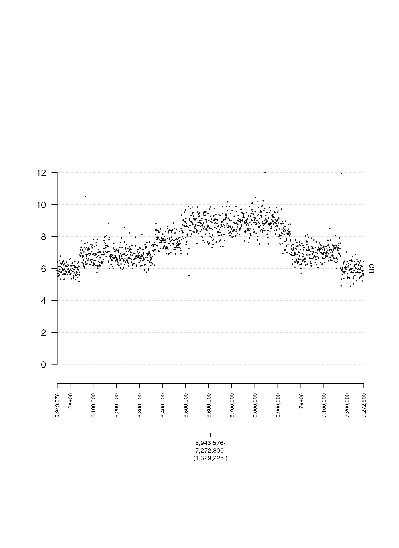
Bar plot
Next, we will plot the same data as a bar plot. To do this, we will
set the parameter bars to TRUE.
coverage.bars.gt <- gTrack(coverage.gr, y.field = "cn", bars = TRUE, y0 = 0, y1 = 12)

plot(coverage.bars.gt, fp + 1e5)
Line plot
Finally, we will plot these data as a line plot, by setting
lines to TRUE.
coverage.lines.gt <- gTrack(coverage.gr, y.field = "cn", lines = TRUE, y0 = 0, y1 = 12)

plot(coverage.lines.gt, fp + 1e5)
Multiple plots
A useful feature of gTrack objects is that multiple
tracks can be concatenated to produce stacked subplots, as shown in the
following example. The direction of concatenation is from the bottom up
(so the first gTrack corresponds with the bottom-most
subplot and the final gTrack corresponds with the top-most
subplot).
concatenated.gt <- c(coverage.gt, coverage.bars.gt, coverage.lines.gt)

plot(concatenated.gt, fp + 1e5)
GRangesList
A gTrack can also be created from a
GRangesList. This is desirable when plotting ranges that
are grouped together in some way, such as alignments deriving from a
single read pair.
Unordered GRangesList (default)
In this example, we will create a gTrack from junction-supporting read pairs. Briefly, these are read pairs that form split, gapped, or discordant alignments, hinting at the existence of a genomic rearrangement.
The alignments associated with each read pair are represented by a
single entry in this example’s GRangesList. In the
corresponding gTrack, alignments from the same GRangesList
entry are linked together by a light gray horizontal line, making it
easy for them to be visually associated.
You can see that there are many junction-supporting reads associated
with read depth change points in the coverage gTrack which
makes sense because aberrant adjacencies can produce copy number
variants.
reads <- readRDS(system.file("extdata", "ovcar.subgraph.reads.rds", package = "gTrack"))
reads.gt <- gTrack(reads)

plot(c(coverage.gt, reads.gt), fp + 1e5)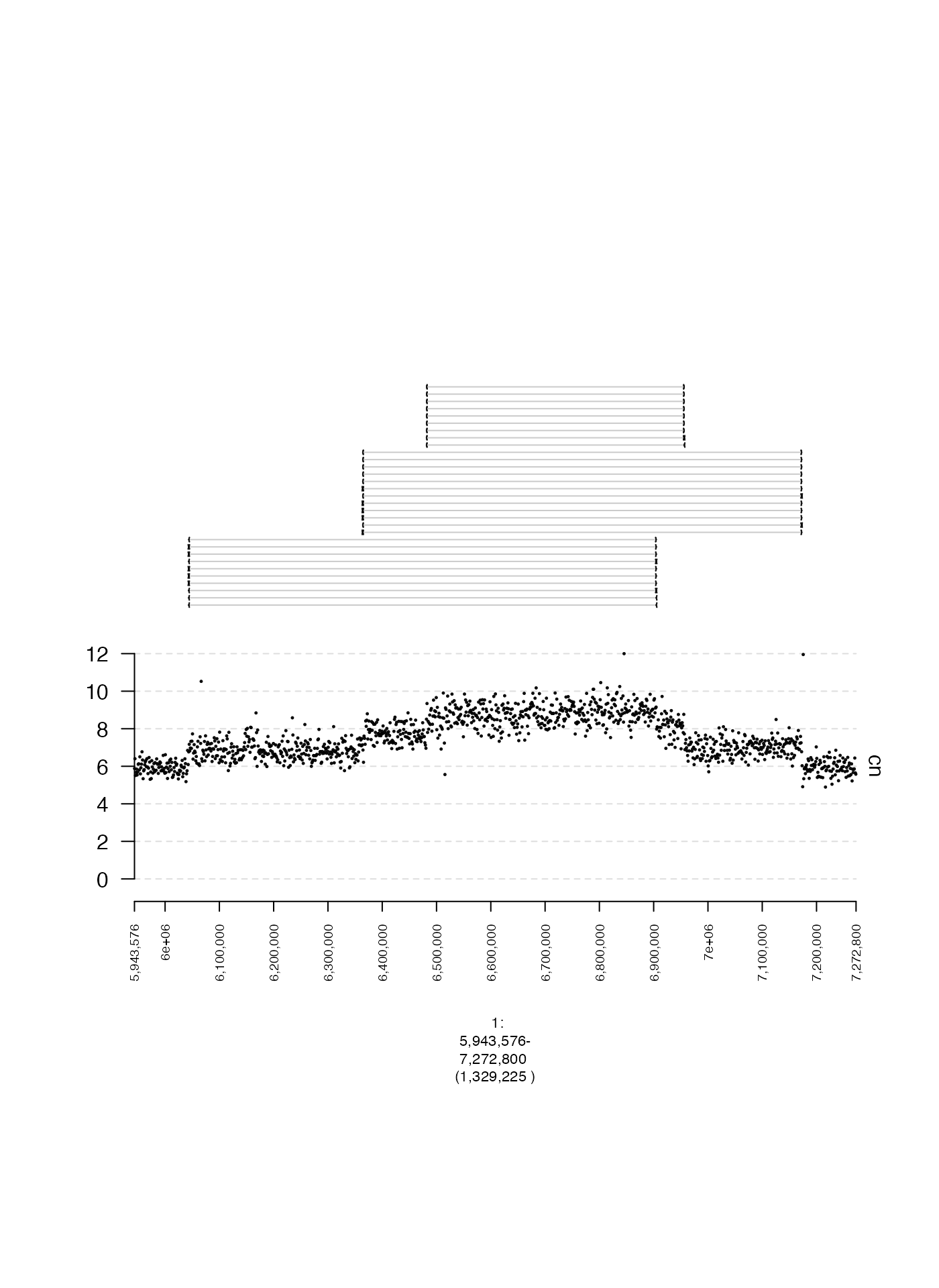
Ordered GRangesList (draw.paths)
Sometimes it is desirable to preserve the ordering of segments within
each GRanges in a GRangesList. For instance, if each GRanges represents
a rearranged somatic haplotype, it is helpful to visualize the exact
order of a rearranged segment. This can be done by setting the parameter
draw.paths to TRUE. Notice the difference
between the plots when this parameter is set!
## create GRangesList for plotting
wks.grl <- readRDS(file.path(project_path, "inst/extdata/ovcar.subgraph.walks.rds"))$grl
fp <- parse.gr("1:6043576-7172800")
paths.gt <- gTrack(wks.grl, draw.paths = TRUE, stack.gap = 1e7, name = "paths")
nopaths.gt <- gTrack(wks.grl, draw.paths = FALSE, stack.gap = 1e7, name = "no paths")

plot(c(nopaths.gt, paths.gt), fp + 5e4)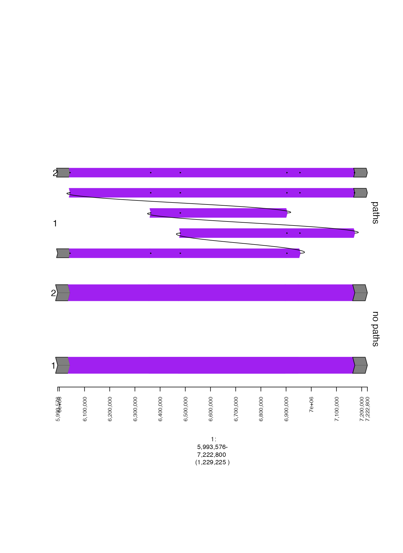
Matrices
Heatmaps (mdata)
A gTrack can be created from a GRanges and
a corresponding adjacency matrix to plot associations between two
genomic ranges. One example of this would be a heatmap, where the color
of each cell is proportional to some value defined by its corresponding
genomic regions.
In this example, we will create a heatmap of the number of shared
read qnames between pairs of genomic intervals. We will
read a GRanges and associated matrix and
create a gTrack from these inputs, which we will plot
alongside the coverage.
As you can see, the off-diagonal elements correspond with copy number change points in the coverage!
mdata.mat <- readRDS(system.file("extdata", "ovcar.subgraph.mdata.mat.rds", package = "gTrack"))
mdata.gr <- readRDS(system.file("extdata", "ovcar.subgraph.mdata.gr.rds", package = "gTrack"))

heatmap.gt <- gTrack(mdata.gr, mdata = mdata.mat, cmap.max = 10)

plot(c(coverage.gt, heatmap.gt), fp + 1e5)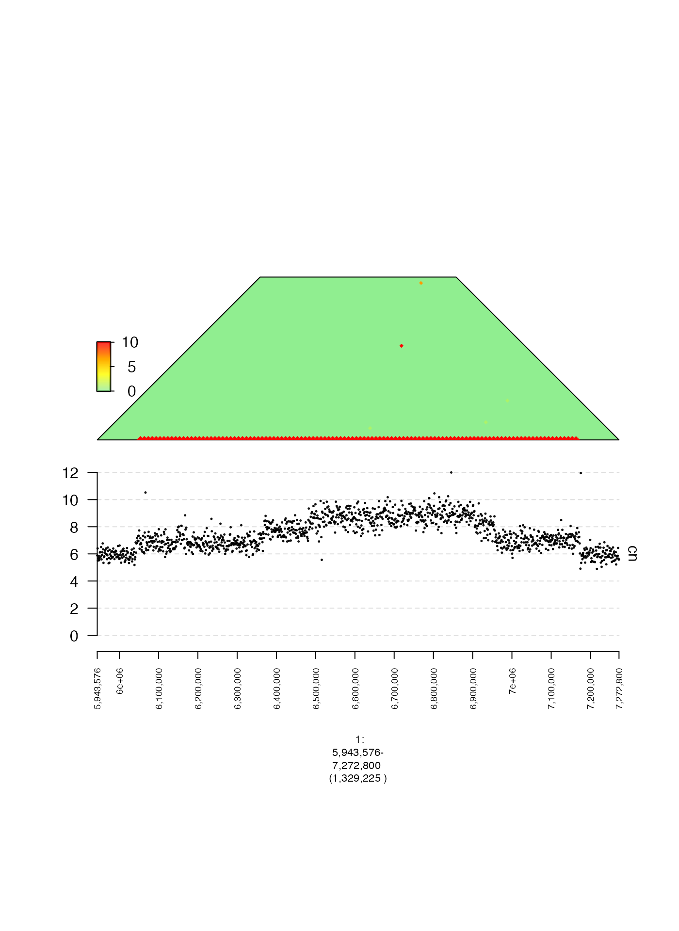
Connections (edges)
Instead of a heatmap, it is also possible to plot the edges between genomic intervals by supplying an adjacency list. In this next example, we will plot edges associated with the off-diagonal squares in the previous heatmap.
edges.dat <- readRDS(system.file("extdata", "ovcar.subgraph.edges.dat.rds", package = "gTrack"))
edges.gr <- readRDS(system.file("extdata", "ovcar.subgraph.edges.gr.rds", package = "gTrack"))

edges.gt <- gTrack(edges.gr, edges = edges.dat)

plot(c(coverage.gt, edges.gt), fp + 1e5)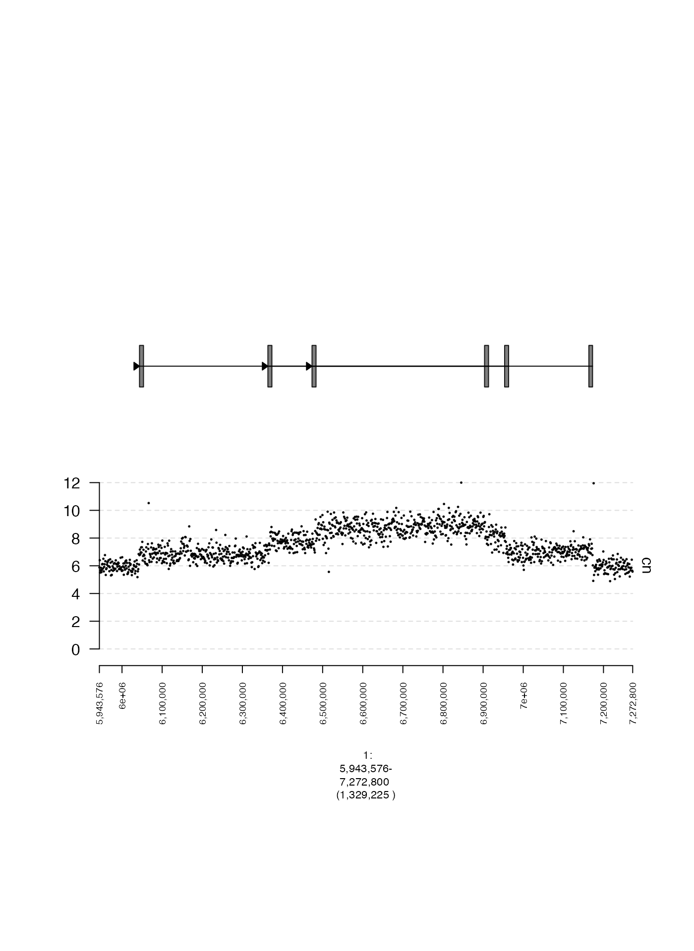
gGraph
gGraphs are genome graphs in which nodes represent
(signed) genomic intervals, and edges represent adjacencies between
those intervals (see our gGnome package here!).
A gTrack can be created from a gGraph using
either the $gt active field or $gtrack method,
as shown below. In this example, we will create a plot of a tumor
gGraph and the associated coverage profile.
gg <- readRDS(system.file("extdata", "ovcar.subgraph.rds", package = "gTrack"))
plot(c(coverage.gt, gg$gt), fp + 1e5)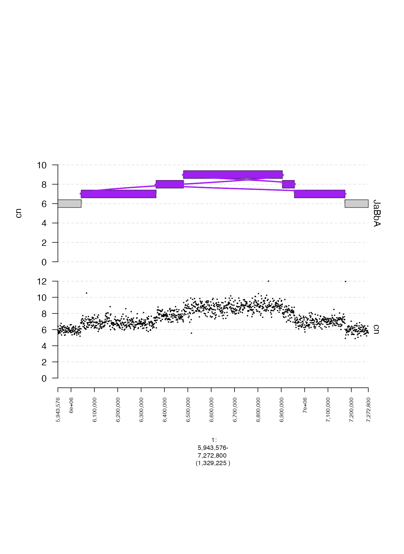
gWalk
gWalks represent paths through a gGraph.
Generally, they represent somatic haplotypes that could exist in a
genome corresponding with a given gGraph (more details in
the gGnome package!). Like gGraphs,
gWalks have active field $gt and method
$gtrack, both of which will produce a
gTrack.
The following example plots a set of gWalks associated
with the gGraph plotted above.
wks <- readRDS(system.file("extdata", "ovcar.subgraph.walks.rds", package = "gTrack"))
plot(c(coverage.gt, gg$gt, wks$gt), fp + 1e5)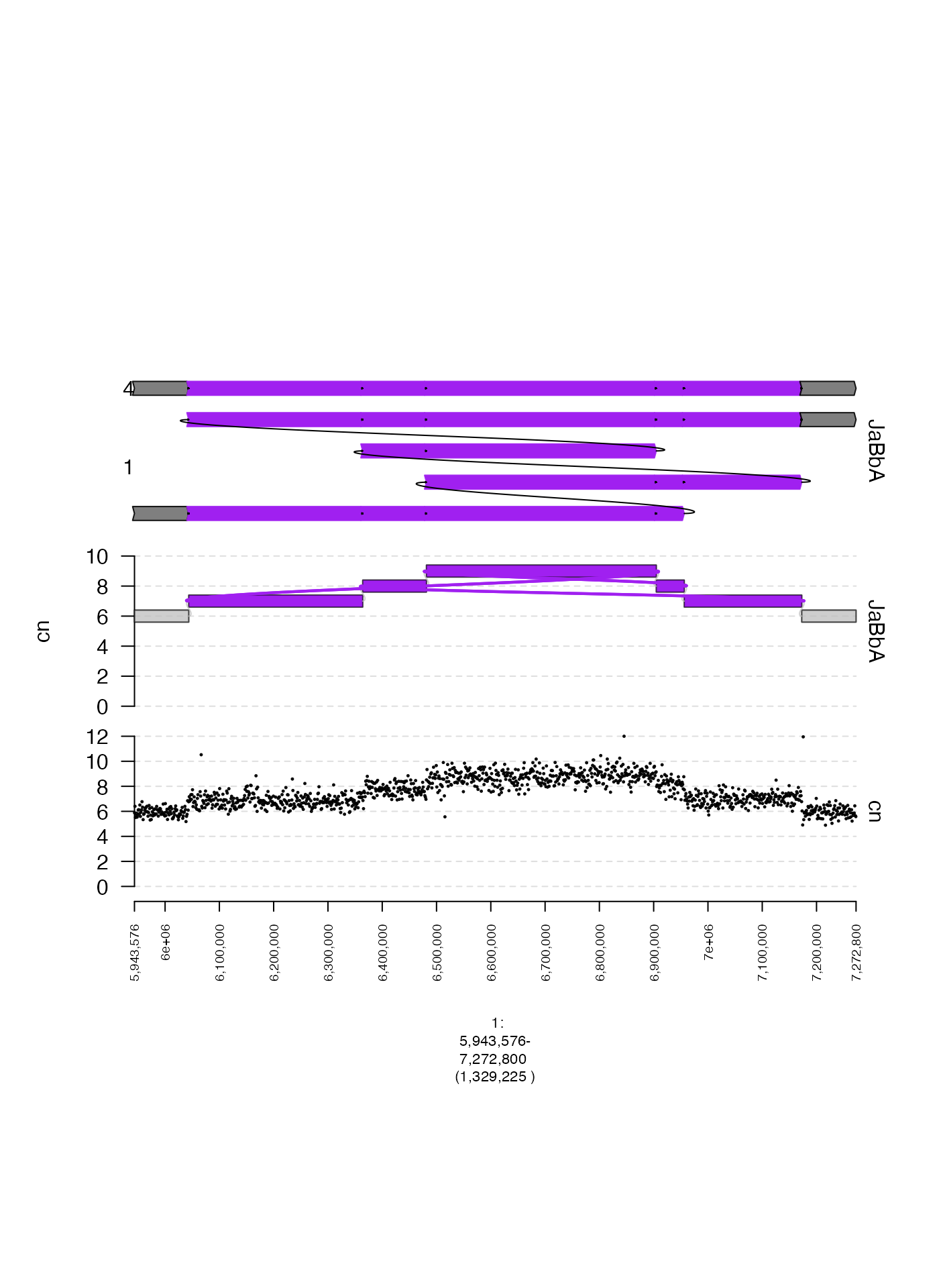
gMatrix
gMatrix is an object implemented in the package
GxG that facilitates analysis and visualization of paired
genomic intervals. There are many use cases for gMatrix,
but the one used in this example is Hi-C data, which consists of read
counts shared by pairs of genomic bins. We will plot the Hi-C profile
associated with this locus.
Again, similar to gWalk and gGraph, a
gTrack can be created for a gMatrix with the
active field $gt or method $gtrack. Here we
will use the $gtrack method to set a parameter for coloring
the heatmap (cmap.max).
gm <- readRDS(system.file("extdata", "ovcar.subgraph.hic.rds", package = "gTrack"))
plot(c(coverage.gt, gg$gt, gm$gtrack(cmap.max = 1000)), fp + 1e5)
Karyogram
You can plot karyograms in gTrack. If no file is passed to the
karyogram method as an argument, it will use the karyogram
datafiles (hg18 or hg19, depending on if the hg19 parameter
is set to FALSE) included with the package. You can specify
if you colored giemsa bands by setting the bands parameter
to TRUE or FALSE (enabled by default). You can
also return the chromosome arms with different colors, and with
centromeres and telemeres marked, by setting arms = TRUE
(also enabled by default)
Here we are plotting the default assembly, hg18, with the bands and arms.
karyogram_fp <- parse.gr("1:1-200000000")
karyogram_gt_hg18 <- karyogram(hg19 = FALSE)
plot(karyogram_gt_hg18, karyogram_fp)
Gencode Tracks
gTrack can also plot a gencode gene track using the
track.gencode method. This method will download the
specified build (indicated by the build parameter) from mskilab.com. You can filter genes by supplying a
character vector to the grep parameter, the
grepe parameter (to exclude genes), or the
genes paramter (to limit the gTrack to only those
genes).
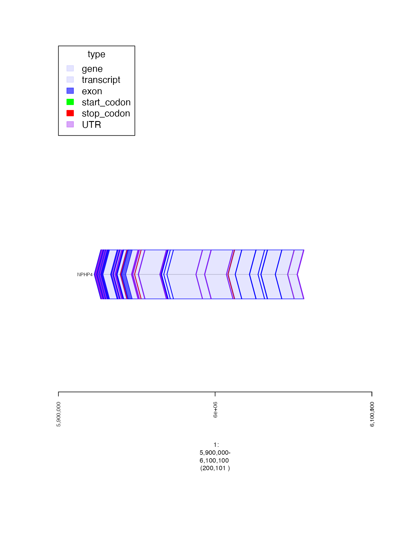
gencode_fp <- parse.gr("1:6000000-6000100")
gencode_gt <- track.gencode(grep = "NPH", grepe = "S2")
expect_error(plot(gencode_gt, gencode_fp + 1e5), NA)