This is a (non-comprehensive) overview of gTrack
parameters that are commonly modified from their default values.
Plotting multiple ranges
Somtimes it is helpful to plot two non-contiguous genomic ranges
side-by-side. This might happen if you’re plotting a structural variant
with breakends that are very distant from each other, or even on
separate chromosomes. This can be done by supplying multiple ranges as
the plotting window as either a GRanges or
GRangesList. The following is an example of a plot with
discontiguous ranges.
coverage.gr = readRDS(system.file("extdata", "ovcar.subgraph.coverage.rds", package = "gTrack"))
coverage.gt = gTrack(coverage.gr, y.field = "cn", circles = TRUE, lwd.border = 0.2, y0 = 0, y1 = 12)

gg = readRDS(system.file("extdata", "ovcar.subgraph.rds", package = "gTrack"))
win = stack(gg$junctions[type == "ALT"]$grl[1])[, c()]
plot(c(coverage.gt, gg$gt), win + 5e4)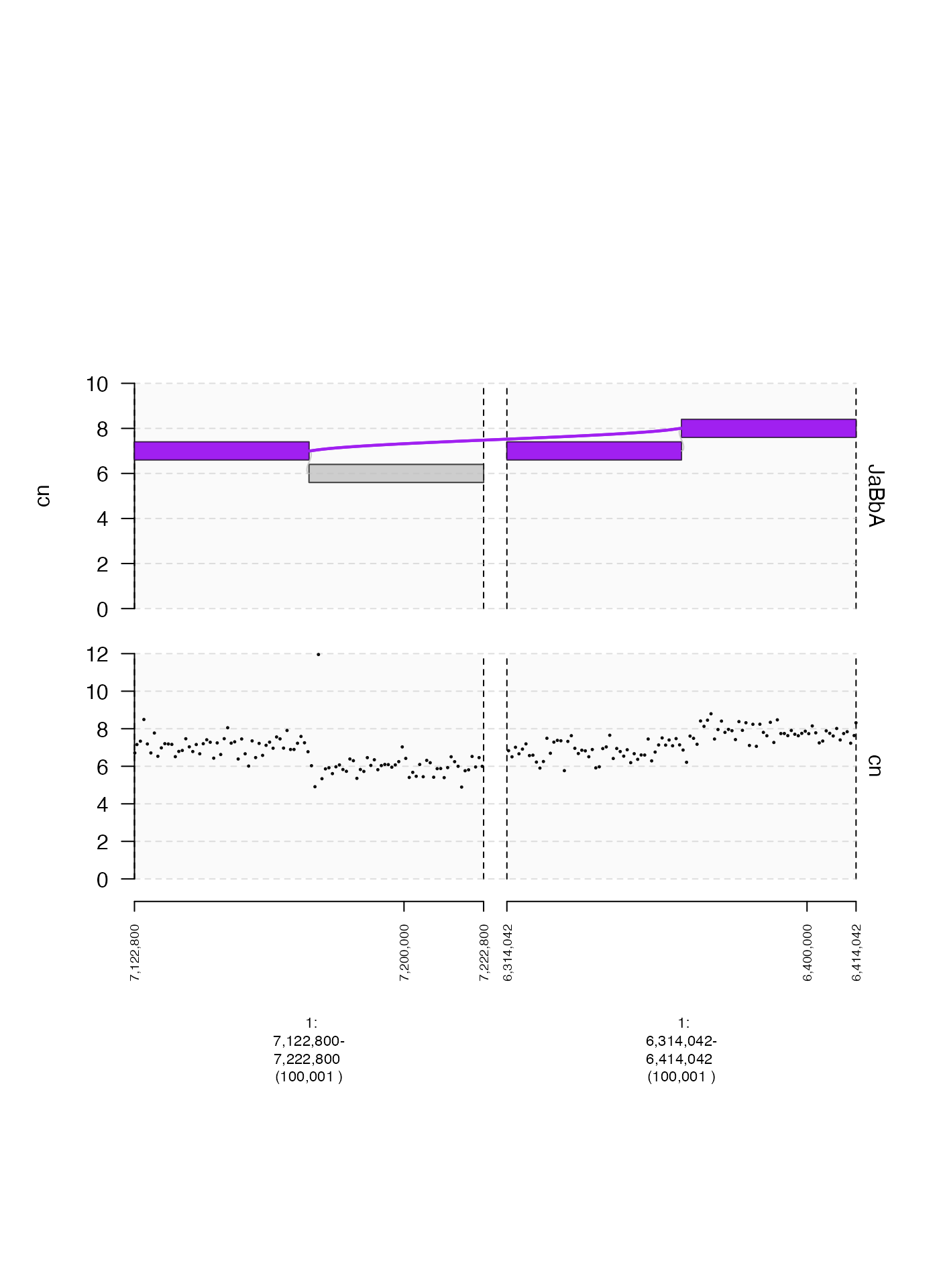
Axes and data
Y-coordinates (y.field)
The x-coordinate of gTrack data is always a genomic
interval. The y-coordinate can be either unspecified, or supplied in a
metadata column of the GRanges or GRangesList.
The name of this metadata column can be specified by supplying a
character string to argument for y.field.
In the following example, we will plot two different metadata fields,
one named foreground and one named cn.
coverage.gr = readRDS(system.file("extdata", "ovcar.subgraph.coverage.rds", package = "gTrack"))

## read depth gTrack without name argument
coverage.cn.gt = gTrack(coverage.gr, y.field = "cn", circles = TRUE, lwd.border = 0.2, y0 = 0, y1 = 12)

## read depth gTrack with name argument
coverage.foreground.gt = gTrack(coverage.gr, y.field = "foreground", circles = TRUE, lwd.border = 0.2, y0 = 0, y1 = 12)

fp = parse.gr("1:6043576-7172800")
plot(c(coverage.cn.gt, coverage.foreground.gt), fp + 1e5)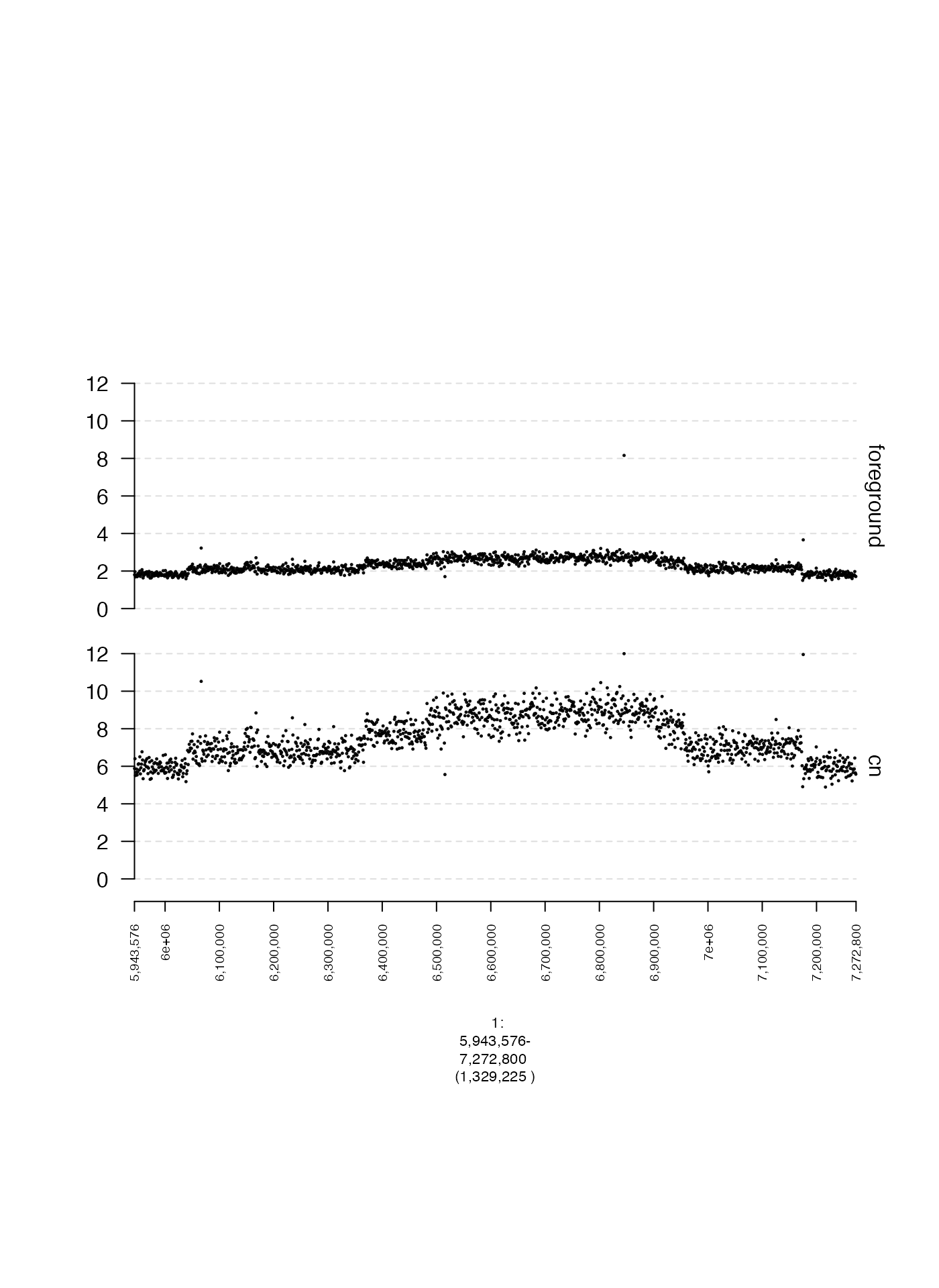
Track names (name)
The name specifies the track label that is shown to the
right of a subplot. Arguments must be character vectors. The default
behavior is to set name to an empty string if
y.field is not specified, and otherwise to set
name to the value passed to y.field. Below is
an example of a scatter plot with and without a name
argument.
coverage.gr = readRDS(system.file("extdata", "ovcar.subgraph.coverage.rds", package = "gTrack"))

## read depth gTrack without name argument
coverage.gt = gTrack(coverage.gr, y.field = "cn", circles = TRUE, lwd.border = 0.2, y0 = 0, y1 = 12)

## read depth gTrack with name argument
coverage.name.gt = gTrack(coverage.gr, name = "coverage", y.field = "cn", circles = TRUE, lwd.border = 0.2, y0 = 0, y1 = 12)

fp = parse.gr("1:6043576-7172800")
plot(c(coverage.gt, coverage.name.gt), fp + 1e5)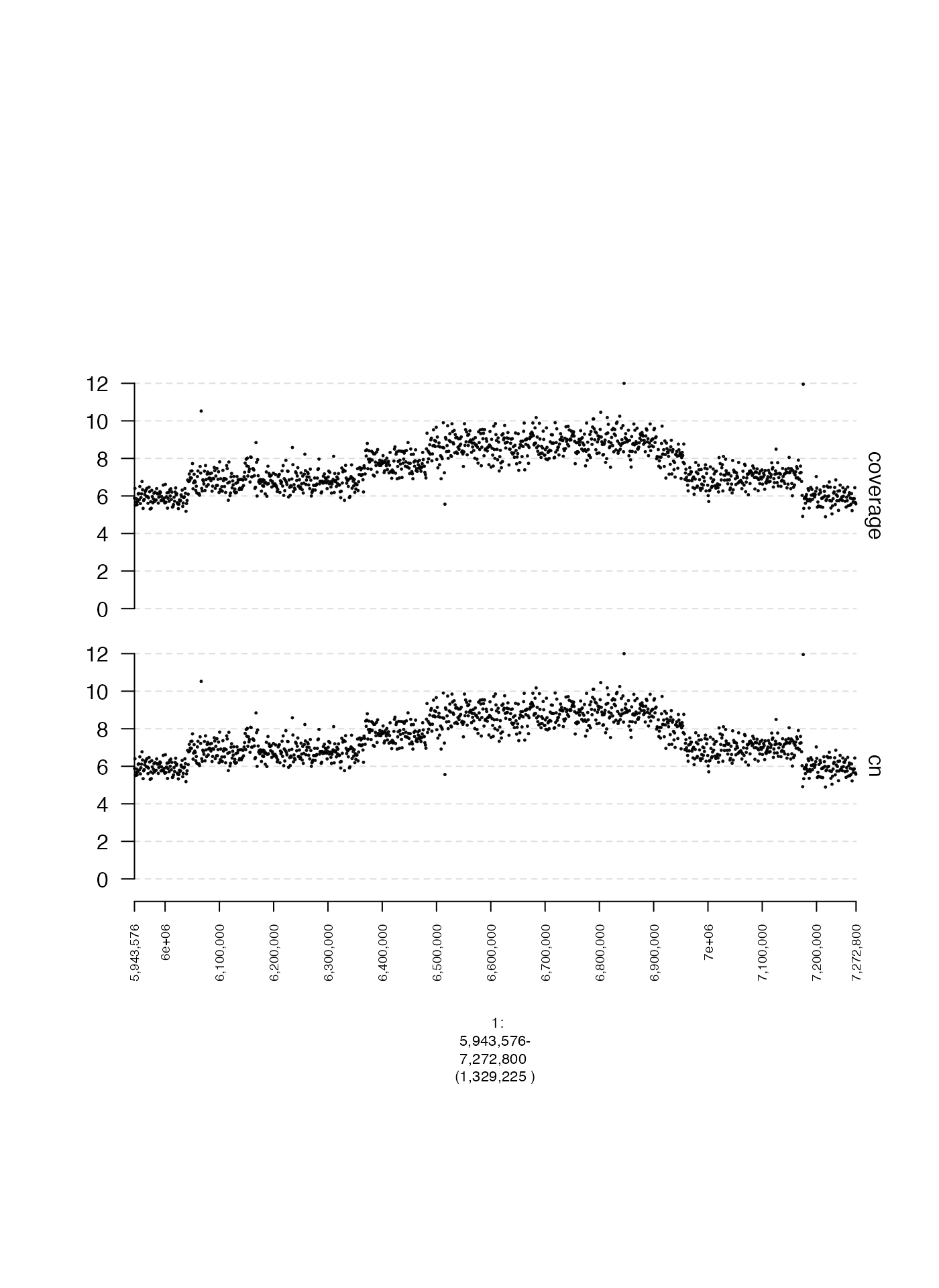
Displaying or hiding the Y-axis (yaxis)
The Y-axis of a gTrack can be toggled on or off entirely
using the logical parameter yaxis, which has default value
TRUE if y.field is specified and
FALSE if not.
Here is an example where yaxis is deliberately set as
FALSE despite suppling a value to y.field.
coverage.gr = readRDS(system.file("extdata", "ovcar.subgraph.coverage.rds", package = "gTrack"))

## read depth gTrack
coverage.gt = gTrack(coverage.gr, y.field = "cn", circles = TRUE, lwd.border = 0.2, y0 = 0, y1 = 12)

## read depth gTrack without Y-axis label
coverage.noy.gt = gTrack(coverage.gr, y.field = "cn", circles = TRUE, lwd.border = 0.2, y0 = 0, y1 = 12, yaxis = FALSE)

fp = parse.gr("1:6043576-7172800")
plot(c(coverage.gt, coverage.noy.gt), fp + 1e5)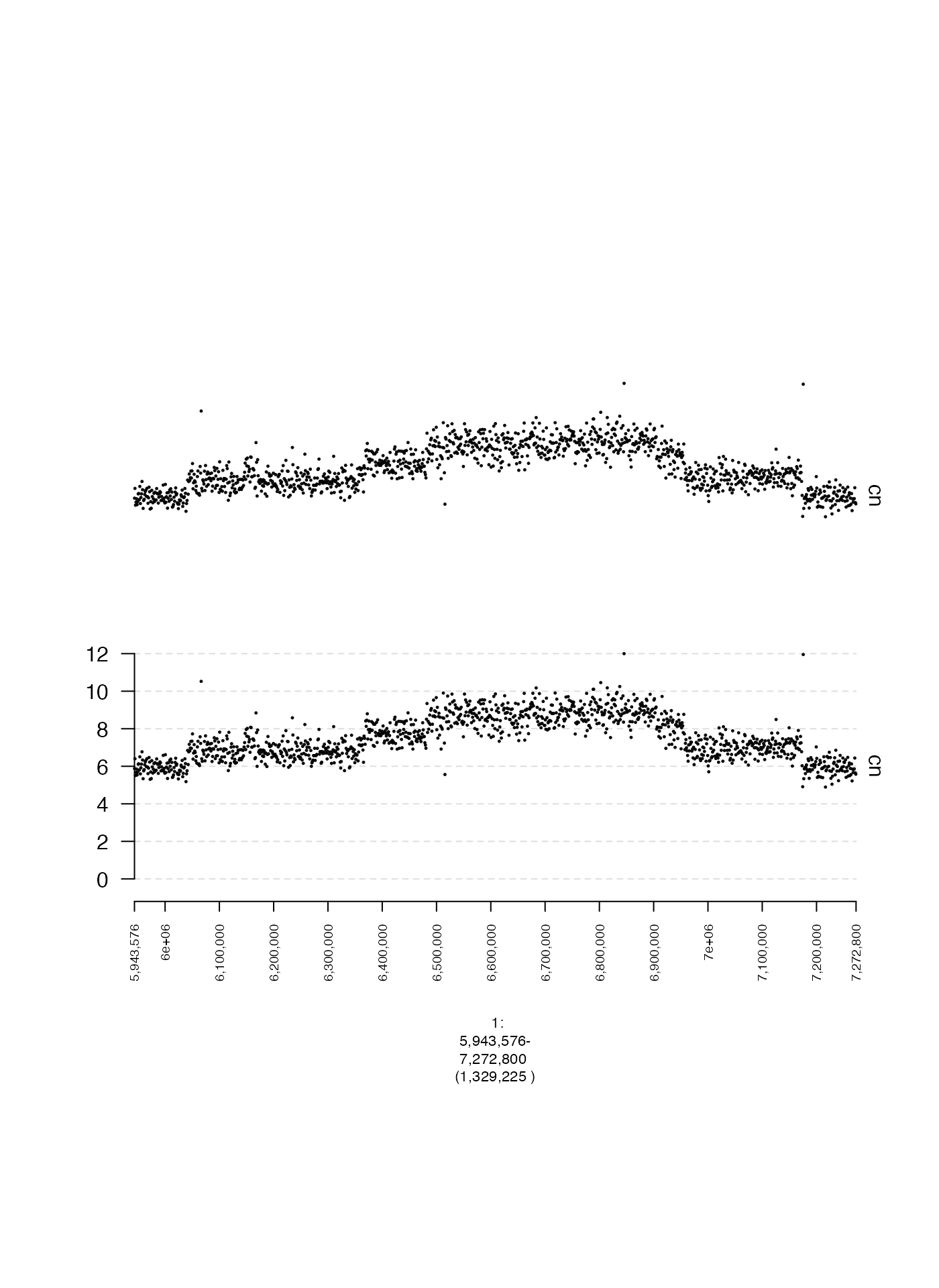
Quantile-based Y-axis cutoffs (y.quantile)
By default, the minimum and maximum y-axis values are determined by
the values of the 1st and 99th percentiles of the data to be plotted.
This percentile can be changed by adjusting y.quantile in
order to plot a wider or narrower range of points. The example below
compares two different values of y.quantile.
coverage.gr = readRDS(system.file("extdata", "ovcar.subgraph.coverage.rds", package = "gTrack"))

## plot points between 1st and 99th percentile
coverage.1.gt = gTrack(coverage.gr, y.field = "cn", circles = TRUE, lwd.border = 0.2, y.quantile = 0.01)

## plot points between 20th and 80th percentile
coverage.20.gt = gTrack(coverage.gr, y.field = "cn", circles = TRUE, lwd.border = 0.2, y.quantile = 0.2)

fp = parse.gr("1:6043576-7172800")
plot(c(coverage.1.gt, coverage.20.gt), fp + 1e5)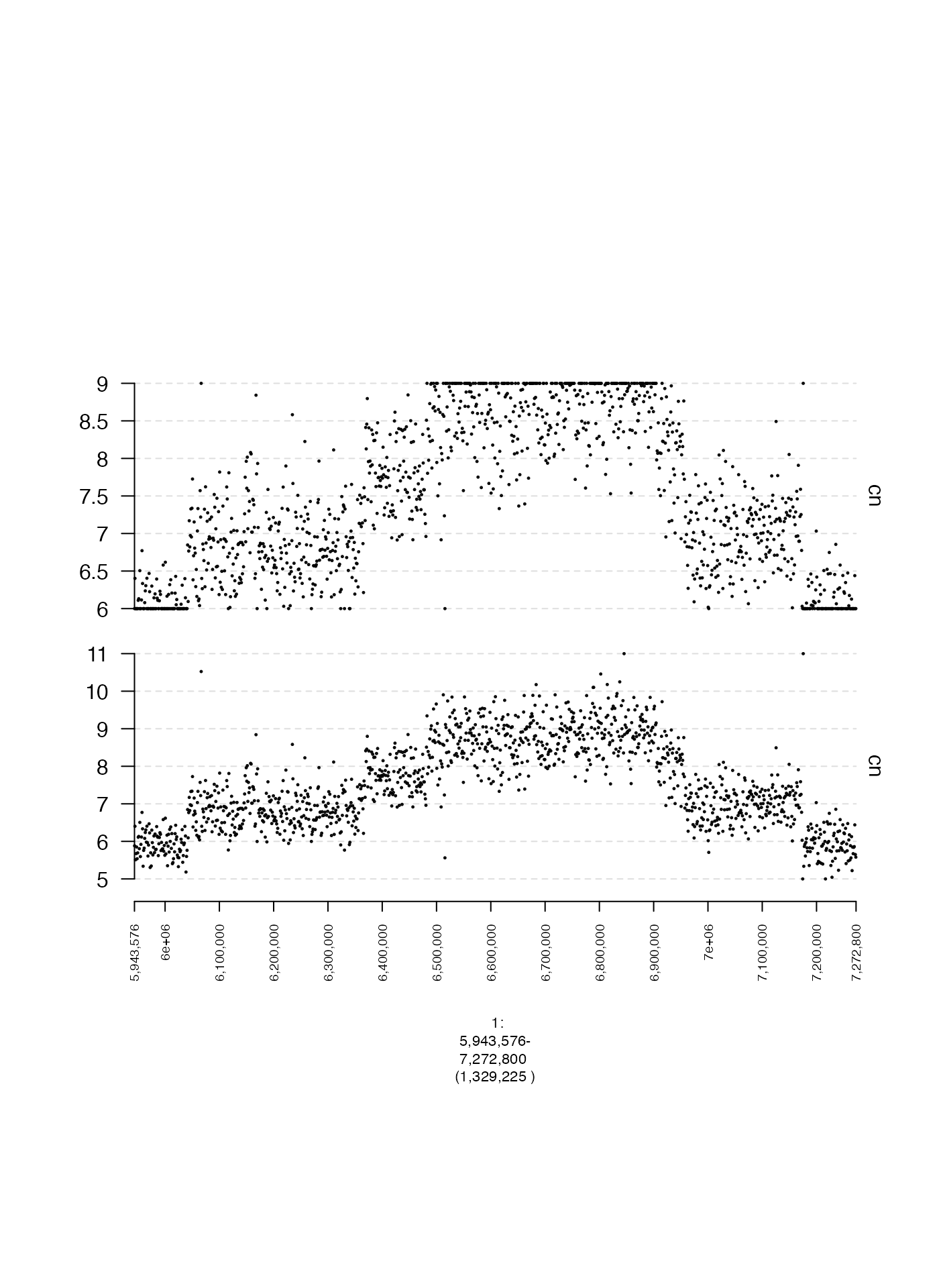
Specifying Y-axis cutoffs (y0 and y1)
The minimum and maximum y-axis values can also be specified directly
with y0 and y1 respectively, which must be
numeric values. Below is an example of the same data with two different
settings for y0 and y1.
coverage.gr = readRDS(system.file("extdata", "ovcar.subgraph.coverage.rds", package = "gTrack"))

## plot points between 0 and 12
coverage.wide.gt = gTrack(coverage.gr, y.field = "cn", circles = TRUE, lwd.border = 0.2, y0 = 0, y1 = 12)

## plot points between 5 and 10
coverage.narrow.gt = gTrack(coverage.gr, y.field = "cn", circles = TRUE, lwd.border = 0.2, y0 = 5, y1 = 10)

fp = parse.gr("1:6043576-7172800")
plot(c(coverage.wide.gt, coverage.narrow.gt), fp + 1e5)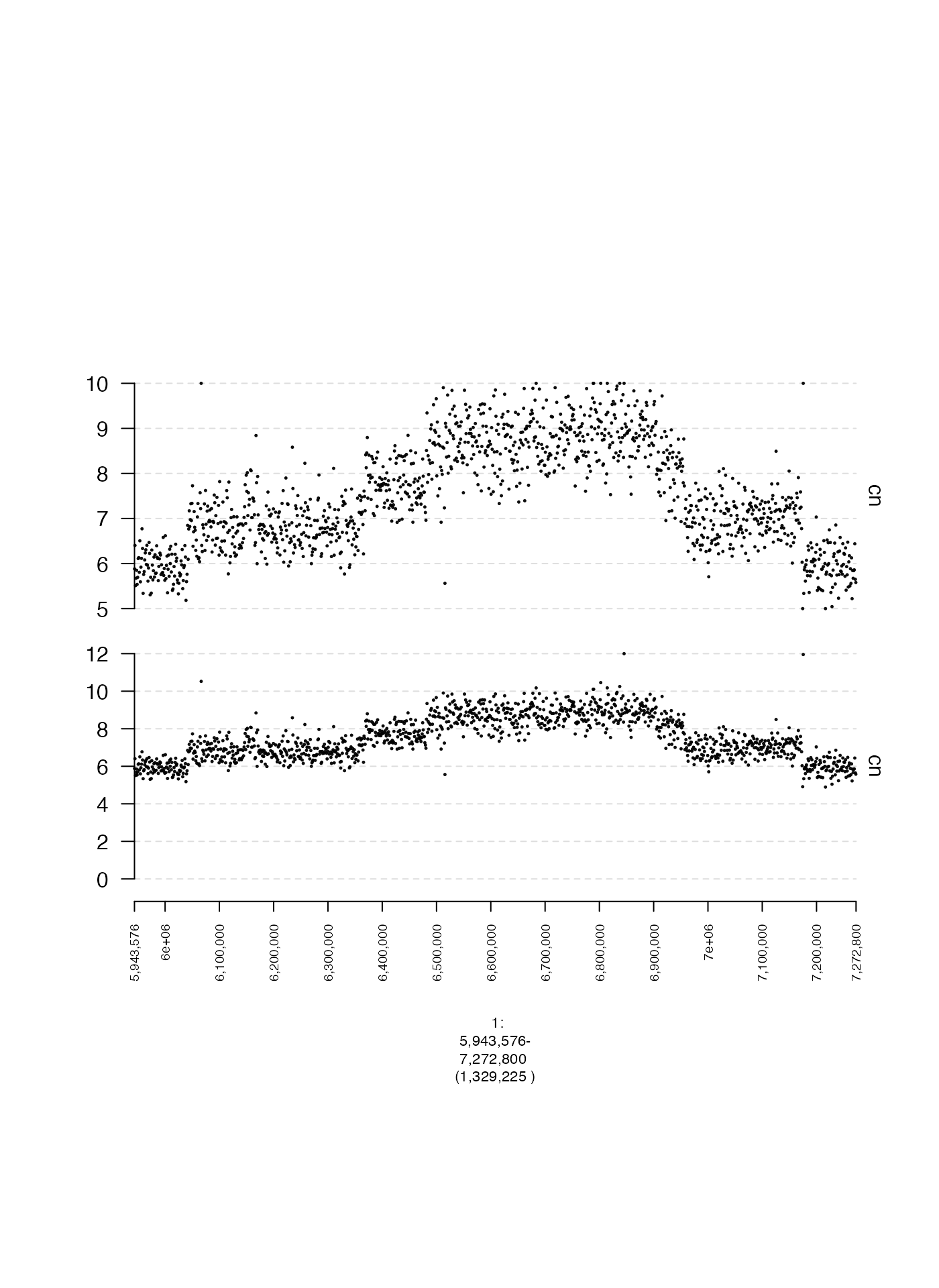
Unbounded Y-axes (y.cap)
Sometimes we may not want to specify limits on the y-coordinates at
all, but rather ensure all points are plotted, regardless of how big or
small they may be. This can be done by setting
y.cap = FALSE as shown in the following example.
coverage.gr = readRDS(system.file("extdata", "ovcar.subgraph.coverage.rds", package = "gTrack"))

## plot points 1st and 99th percentiles (default)
coverage.gt = gTrack(coverage.gr, y.field = "cn", circles = TRUE, lwd.border = 0.2)

## no limits on y
coverage.all.gt = gTrack(coverage.gr, y.field = "cn", circles = TRUE, lwd.border = 0.2, y.cap = FALSE)

fp = parse.gr("1:6043576-7172800")
plot(c(coverage.gt, coverage.all.gt), fp + 1e5)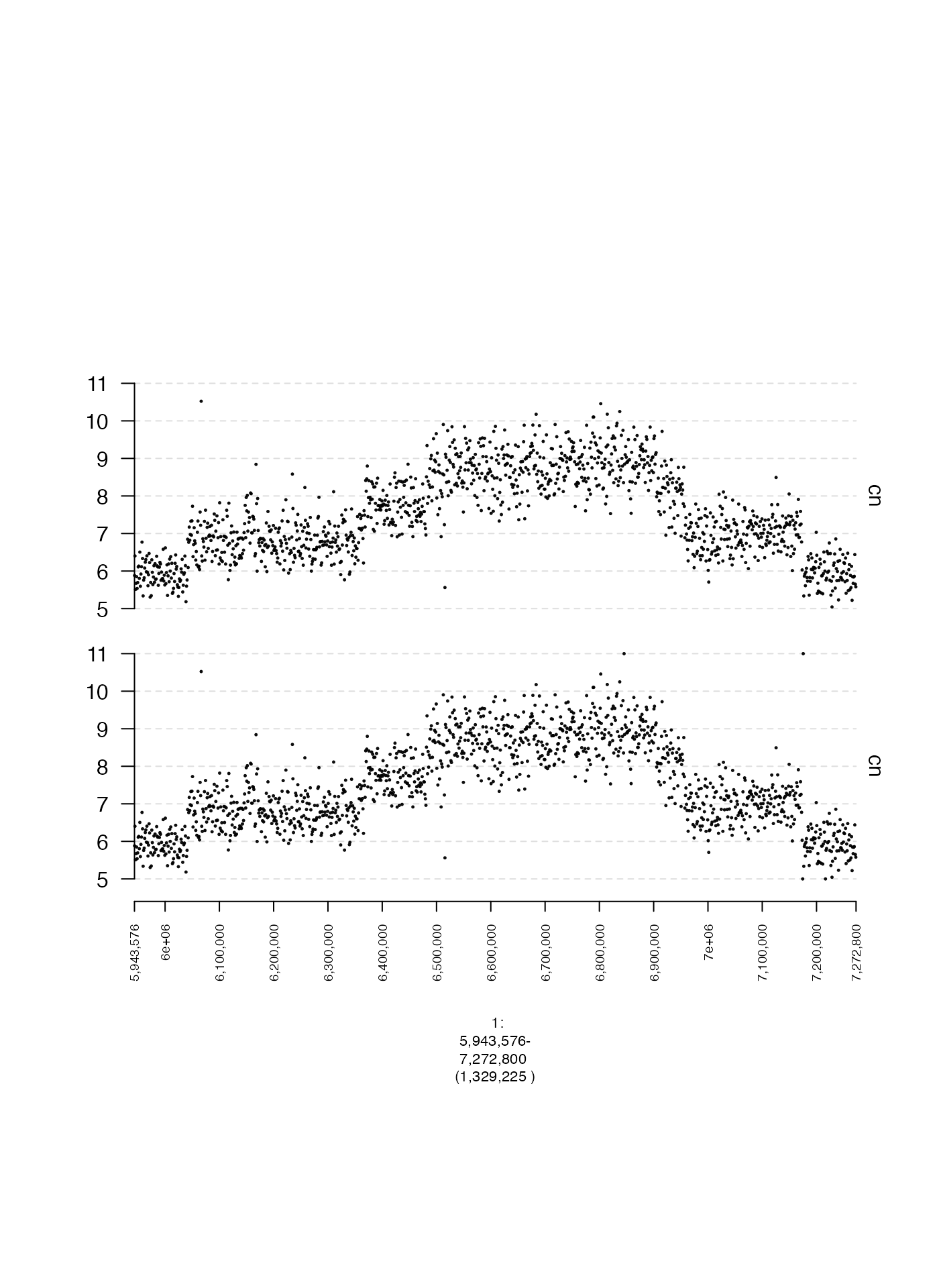
Point density and spacing
Stacking adjacent ranges (stack.gap)
Sometimes closely spaced genomic intervals can be difficult to
discern. If no y-coordinate is specified, sometimes it is helpful to
stagger these intervals vertically to make them more visually distinct.
This can be done by setting the parameter stack.gap to some
numeric value. This will vertically stack adjacent intervals separated
by a genomic distance (in base pairs) below that value.
## create tiled genomic intervals
win = GRanges(seqnames = "1", ranges = IRanges(start = 1, width = 1e5))
tiles = gUtils::gr.tile(win, width = 1e4)

## gTrack without vertical staggering
tiles.gt = gTrack(tiles, name = "original")

## stack intervals within 1 Kbp of each other
tiles.stack.gt = gTrack(tiles, stack.gap = 1000, name = "stacked")

plot(c(tiles.gt, tiles.stack.gt), win)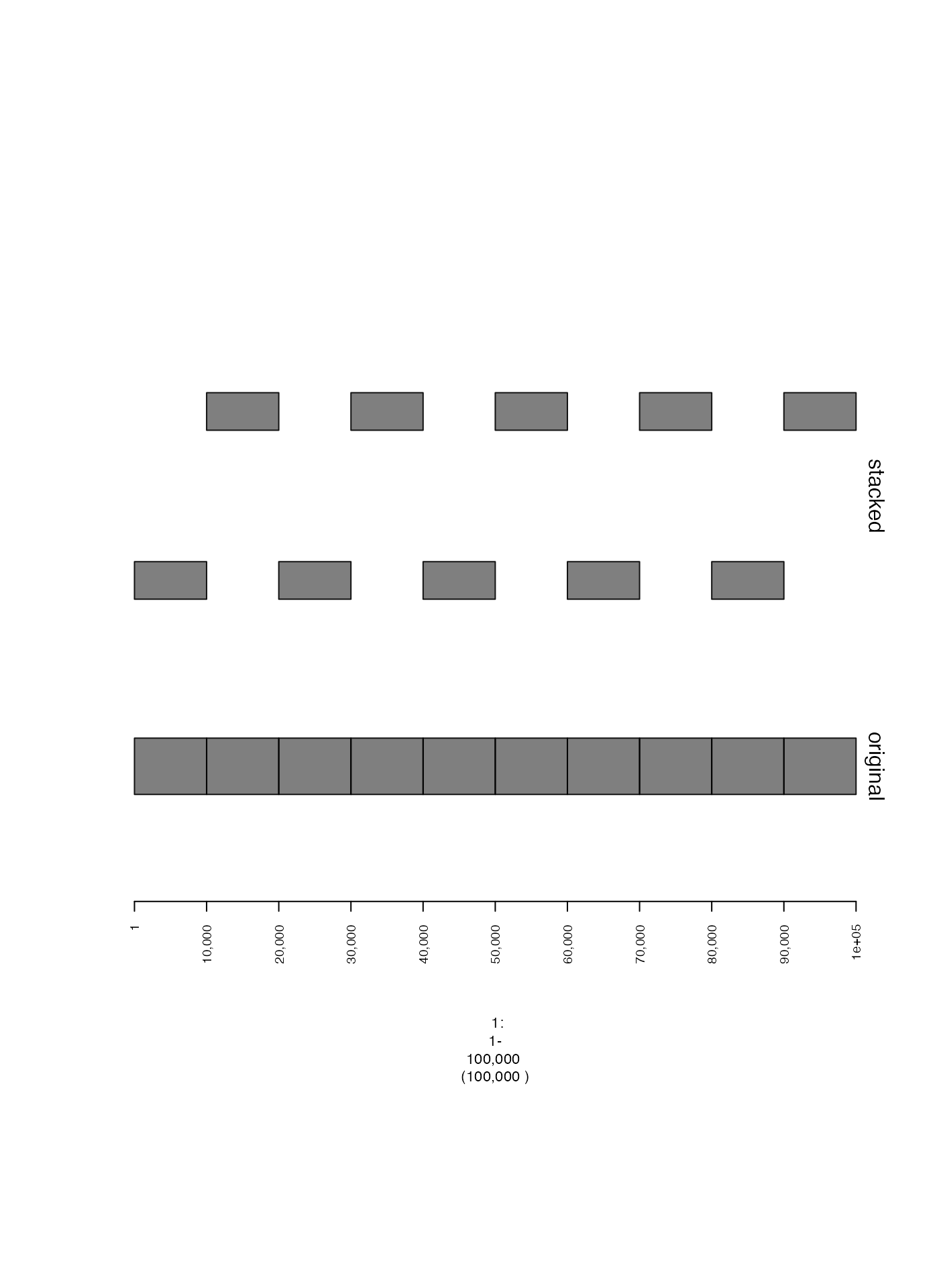
Number of plotted ranges (max.ranges)
A gTrack with a huge number of genomic intervals can
take a long time to plot, and if there are many overlapping points it
doesn’t make sense to include all of them. To downsample points, you can
set max.ranges to some number, which will only plot that
number of randomly selected points.
coverage.gr = readRDS(system.file("extdata", "ovcar.subgraph.coverage.rds", package = "gTrack"))

## plot everything
coverage.gt = gTrack(coverage.gr, y.field = "cn", circles = TRUE, lwd.border = 0.2, name = "original")

## only plot 50 points
coverage.downsample.gt = gTrack(coverage.gr, y.field = "cn", circles = TRUE, lwd.border = 0.2, max.ranges = 50, name = "downsampled")

fp = parse.gr("1:6043576-7172800")
plot(c(coverage.gt, coverage.downsample.gt), fp + 1e5)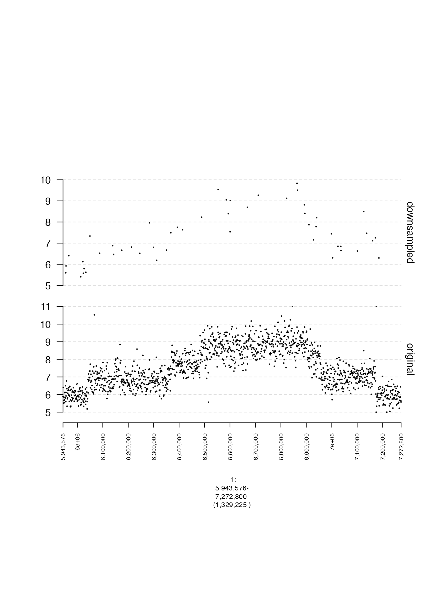
Data labels
By default, named GRanges and GRangesList
are labeled in gTrack. This behavior is illustrated in the
following example.
## define plotting window
win = GRanges(seqnames = "1", ranges = IRanges(start = 1, width = 1e5))

## create named GRanges
gr = GRanges(seqnames = "1", ranges = IRanges(start = c(1, 50001), width = 1e3), strand = "+", other_labels = c("C", "D"))
names(gr) = c("A", "B")

## create gTrack
gt = gTrack(gr, name = "original")

plot(c(gt), win)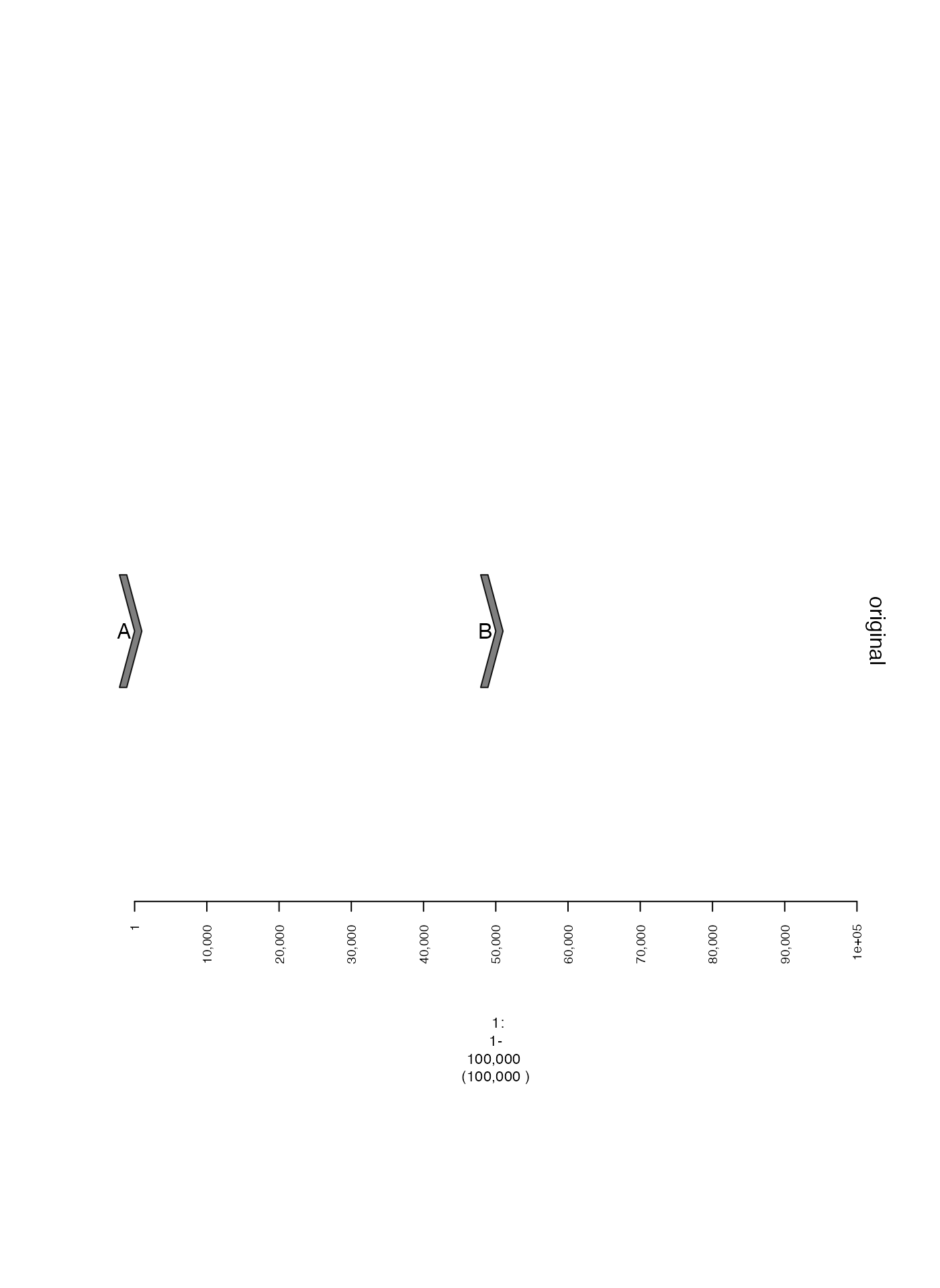
Suppressing labels
These labels can be hidden by setting labels.suppress to
TRUE. If you want to specifically supress labels of a
GRanges or GRangesList, you can also use
labels.suppress.gr or labels.suppress.grl.
## create gTrack with no labels
nolabels.gt = gTrack(gr, labels.suppress = TRUE, name = "no labels")

plot(c(gt, nolabels.gt), win)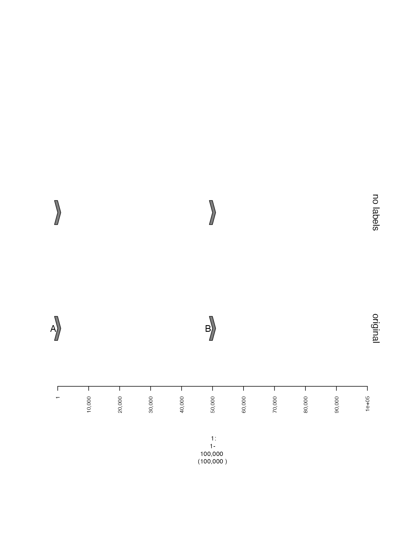
Specifying labels
Labels can also be specified in a metadata column of a
GRanges or GRangesList. To use these labels,
the name of the relevant column should be passed as an argument for
gr.labelfield or grl.labelfield, as seen in
the example below. These will appear in the middle of the GRanges
instead of on the left.
otherlabels.gt = gTrack(gr, gr.labelfield = "other_labels", name = "other labels", labels.suppress = TRUE)

plot(c(gt, otherlabels.gt), win)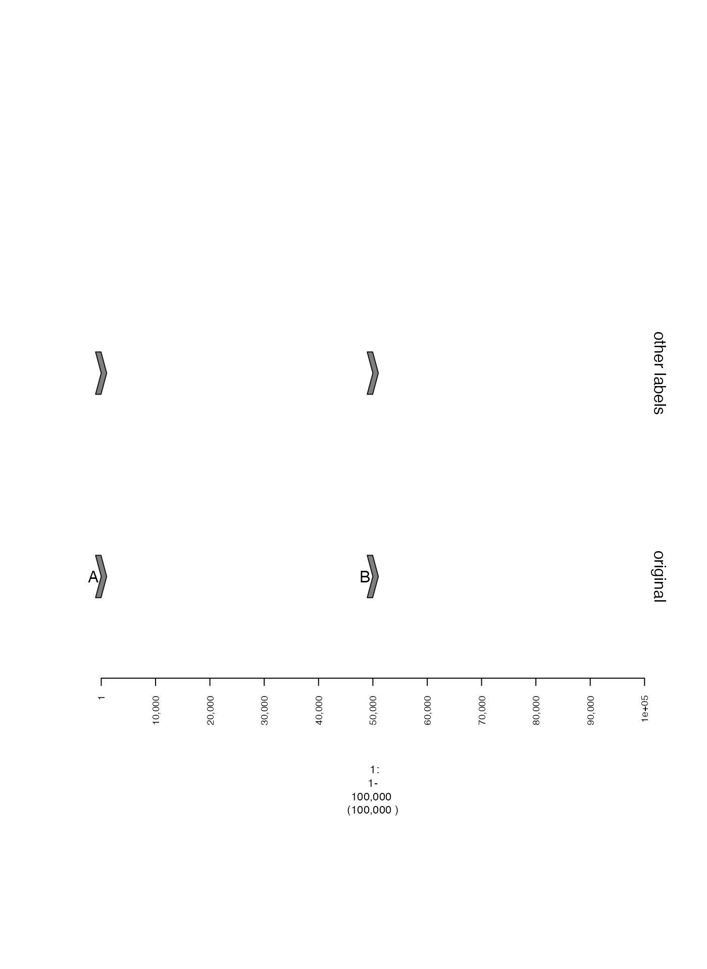
Point and line style
Scatterplot point size (lwd.border)
The size of points in a scatterplot can be controlled by
lwd.border with larger values producing larger points. Here
is an illustrative example.
coverage.gr = readRDS(system.file("extdata", "ovcar.subgraph.coverage.rds", package = "gTrack"))

## two gTracks with slightly different point sizes
coverage.small.gt = gTrack(coverage.gr, y.field = "cn", circles = TRUE, lwd.border = 0.2, y0 = 0, y1 = 12, name = "small")
coverage.big.gt = gTrack(coverage.gr, y.field = "cn", circles = TRUE, lwd.border = 0.5, y0 = 0, y1 = 12, name = "big")

fp = parse.gr("1:6043576-7172800")
plot(c(coverage.small.gt, coverage.big.gt), fp + 1e5)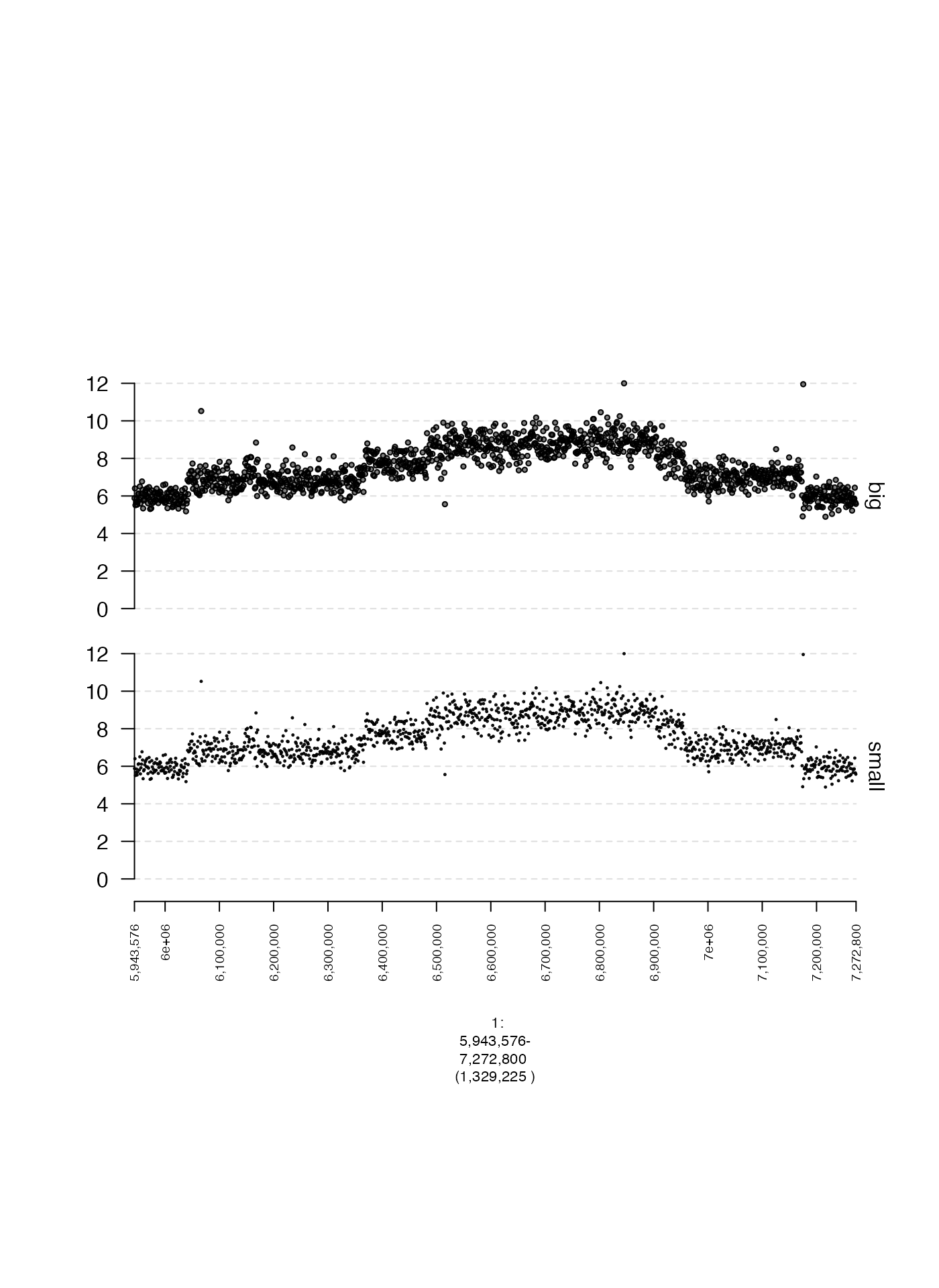
Width of plotted ranges (ywid)
The thickness of plotted segments can be adjusted using the
ywid parameter.
win = GRanges(seqnames = "1", ranges = IRanges(start = 1, width = 1e5))

## create named GRanges
gr = GRanges(seqnames = "1", ranges = IRanges(start = c(1, 50001), width = 1e4), strand = "+", cn = c(1,2), labs = c("A", "B"))

## create gTrack
narrow.gt = gTrack(gr, name = "narrow", ywid = 0.3)
wide.gt = gTrack(gr, name = "wide", ywid = 0.5)

plot(c(narrow.gt, wide.gt), win)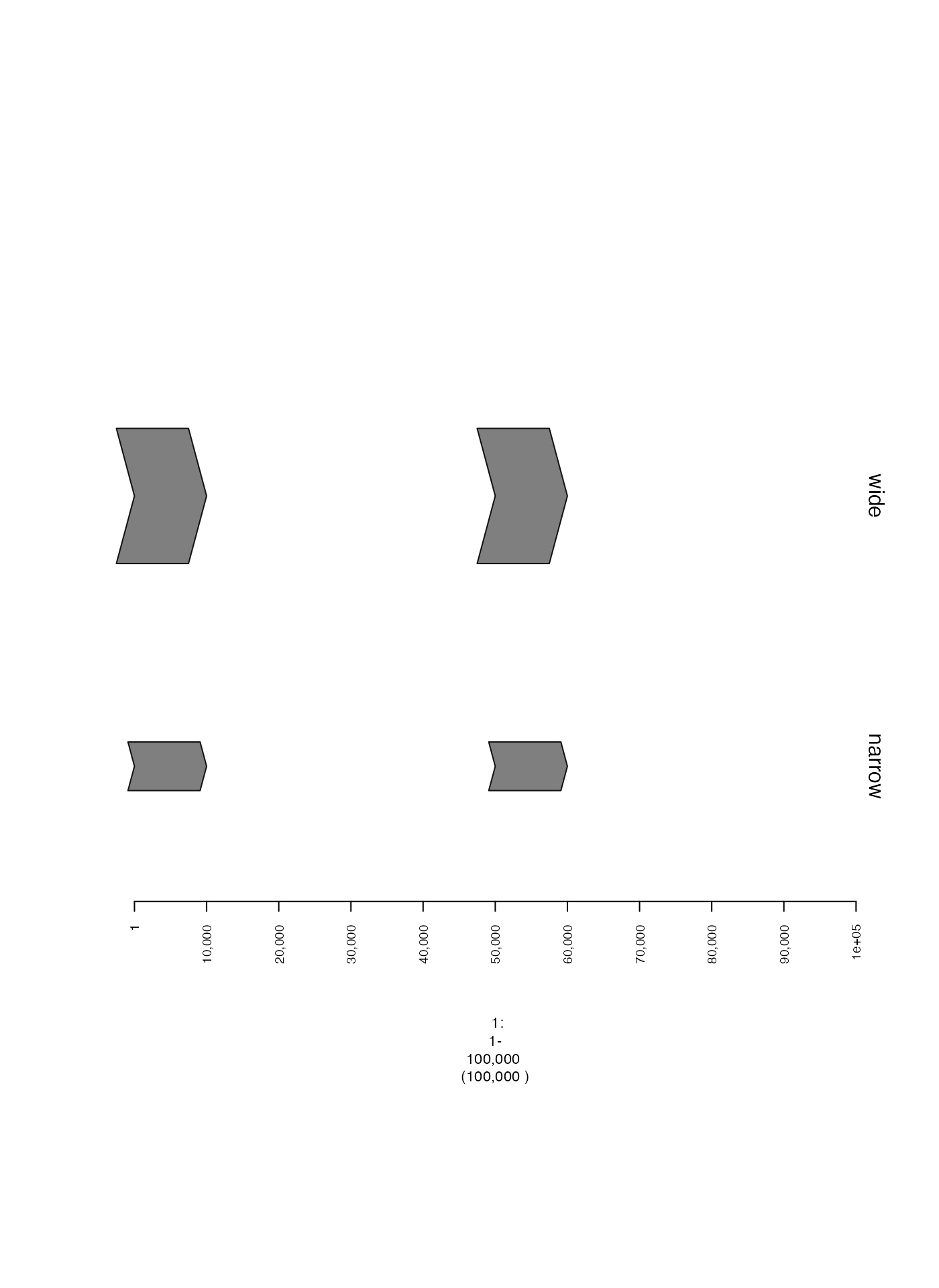
Alternatively, by adjusting the ywid metadata column of
supplied GRanges, the width of each range can be adjusted
individually.
win = GRanges(seqnames = "1", ranges = IRanges(start = 1, width = 1e5))

## create named GRanges
gr = GRanges(seqnames = "1", ranges = IRanges(start = c(1, 50001), width = 1e4), strand = "+", cn = c(1,2), labs = c("A", "B"), ywid = c(0.3, 0.5))

## create gTrack
gt = gTrack(gr, name = "narrow", gr.labelfield = "labs")

plot(c(gt), win)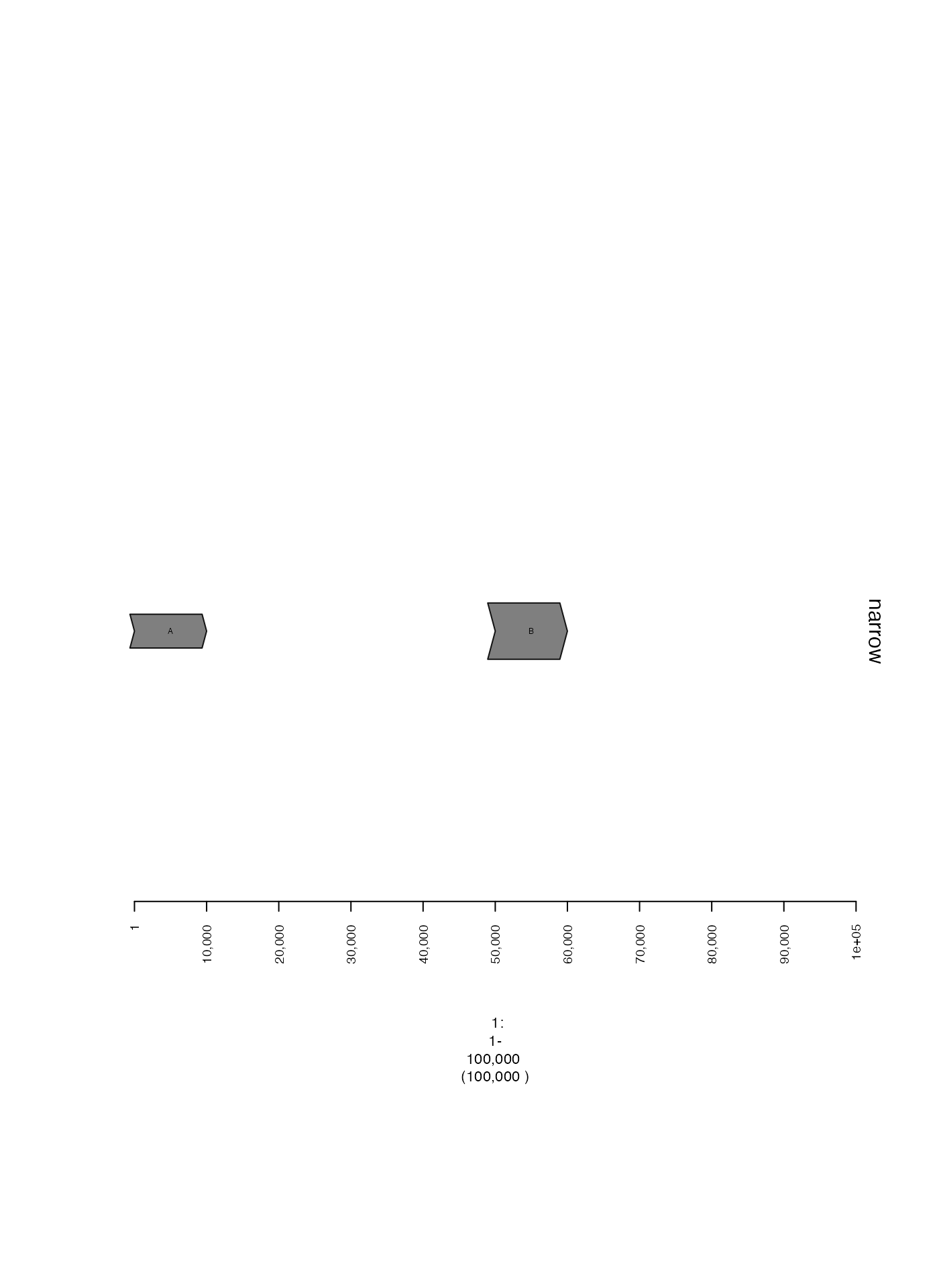
Colors
Specifying data color directly (col)
If col is a metadata column of the GRanges
or GRangesList used to construct a gTrack and contains
colors (either in hexadecimal form or as character vectors) then these
values determine the color of the plotted point. Here is an example,
where points within 10 Kbp of a junction breakend are colored in
red.
coverage.gr = readRDS(system.file("extdata", "ovcar.subgraph.coverage.rds", package = "gTrack"))
gg = readRDS(system.file("extdata", "ovcar.subgraph.rds", package = "gTrack"))

values(coverage.gr)[, "near_breakend"] = ifelse(coverage.gr %^% (stack(gg$junctions[type == "ALT"]$grl) + 1e4), "yes", "no")
values(coverage.gr)[, "col"] = ifelse(values(coverage.gr)[, "near_breakend"] == "yes", "red", "black")

coverage.col.gt = gTrack(coverage.gr, y.field = "cn", circles = TRUE, lwd.border = 0.2, y0 = 0, y1 = 12)

fp = parse.gr("1:6043576-7172800")
plot(c(coverage.col.gt, gg$gt), fp + 1e5)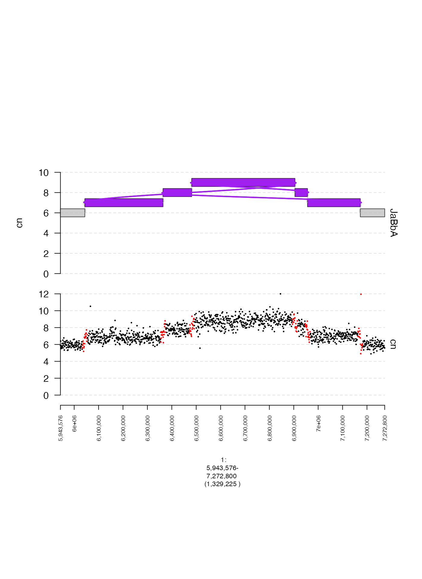
Coloring by secondary label (gr.colorfield and grl.colorfield)
We can also map discrete values in a metadata column in to colors
automatically. Here is one example, using values in
near_breakend. Here, gr.colorfield is set to
"near_breakend" indicating that the gTrack
should color points according to their value in this column. For
GRangesList the analogous parameter
grl.colorfield should be modified.
coverage.col.gt = gTrack(coverage.gr, y.field = "cn", circles = TRUE, lwd.border = 0.2, y0 = 0, y1 = 12, gr.colorfield = "near_breakend")

fp = parse.gr("1:6043576-7172800")
plot(c(coverage.col.gt, gg$gt), fp + 1e5)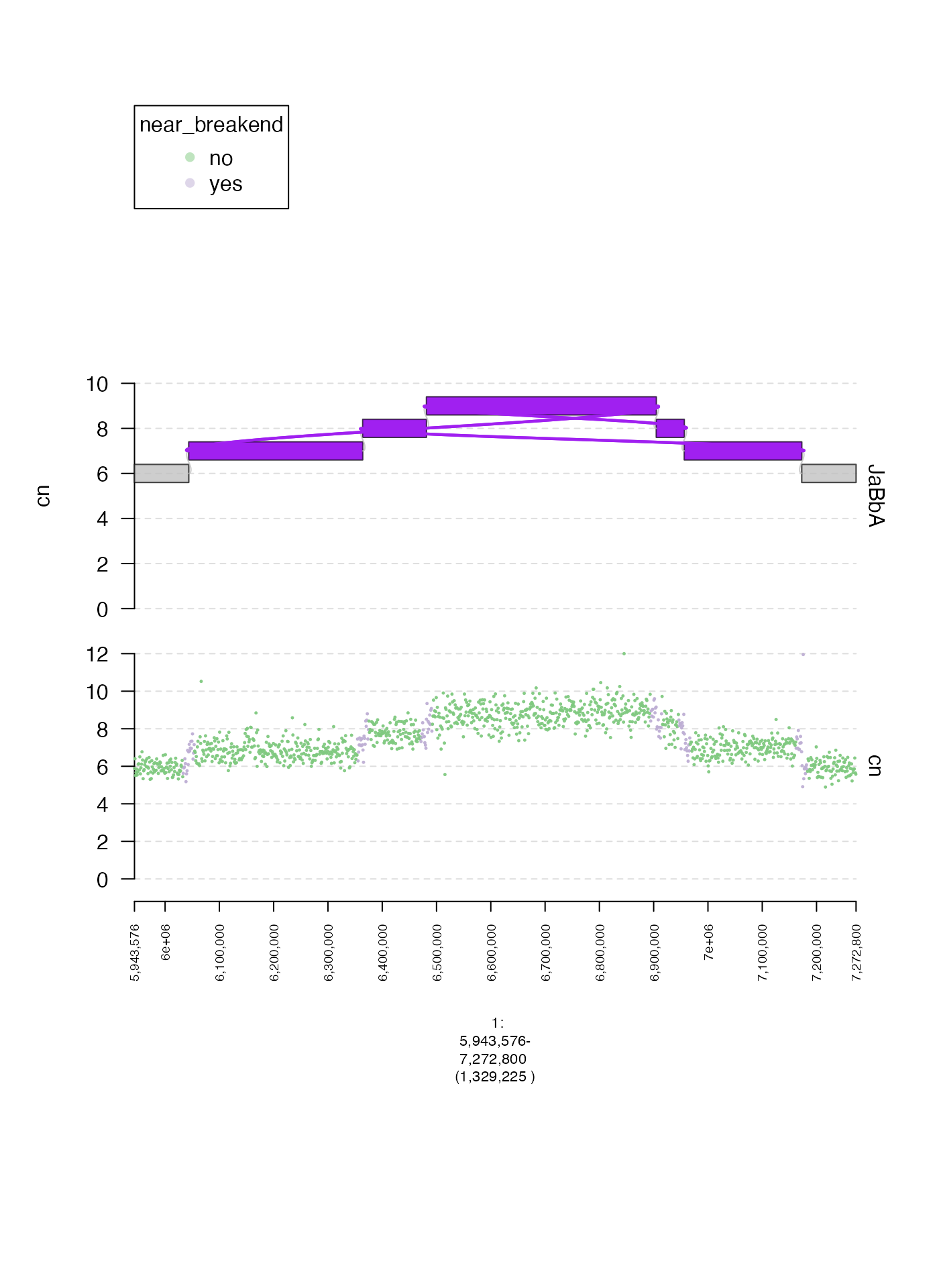
Custom map from label to color (colormaps)
When using gr.colorfield we can also supply a custom map
of labels to colors by passing a named vector to colormap.
Here is one illustrative example.
coverage.col.gt = gTrack(coverage.gr, y.field = "cn", circles = TRUE, lwd.border = 0.2, y0 = 0, y1 = 12, gr.colorfield = "near_breakend", colormap = c("yes" = "red", "no" = "blue"))

fp = parse.gr("1:6043576-7172800")
plot(c(coverage.col.gt, gg$gt), fp + 1e5)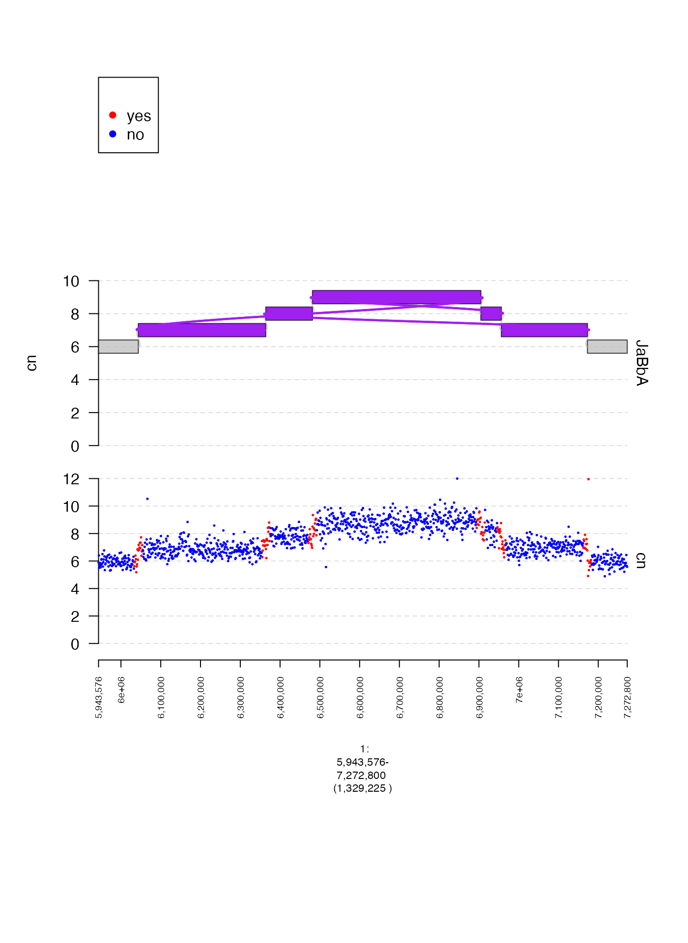
Background color (bg.col)
We can change the background color of our gTrack using the
bg.col param. Here is an example where the background is
set to blue.
coverage.col.gt = gTrack(coverage.gr, y.field = "cn", circles = TRUE, lwd.border = 0.2, y0 = 0, y1 = 12, col = "black", bg.col = alpha("blue", 0.1))

fp = parse.gr("1:6043576-7172800")
plot(c(coverage.col.gt, gg$gt), fp + 1e5)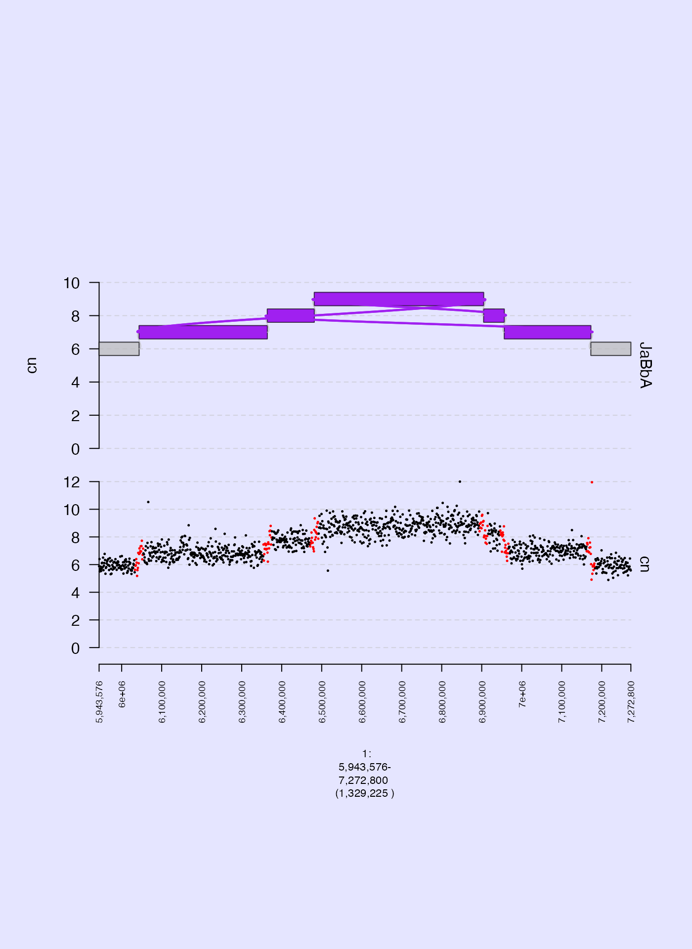
Color thresholds (cmap.max and cmap.min)
When plotting matrix and gMatrix heatmaps
it is sometimes useful to set thresholds for mapping numerical values to
the color gradient. cmap.min is the minimum number, under
which the gradient is not applied, and cmap.max is the
maximum number to which the gradient is applied. Below, I plot two
examples, with different ranges for these parameters.
gm = readRDS(system.file("extdata", "ovcar.subgraph.hic.rds", package = "gTrack"))
fp = parse.gr("1:6043576-7172800")
plot(c(gm$gtrack(cmap.min = 0, cmap.max = 1000, name = "wide"), gm$gtrack(cmap.min = 200, cmap.max = 300, name = "narrow")), fp + 1e5)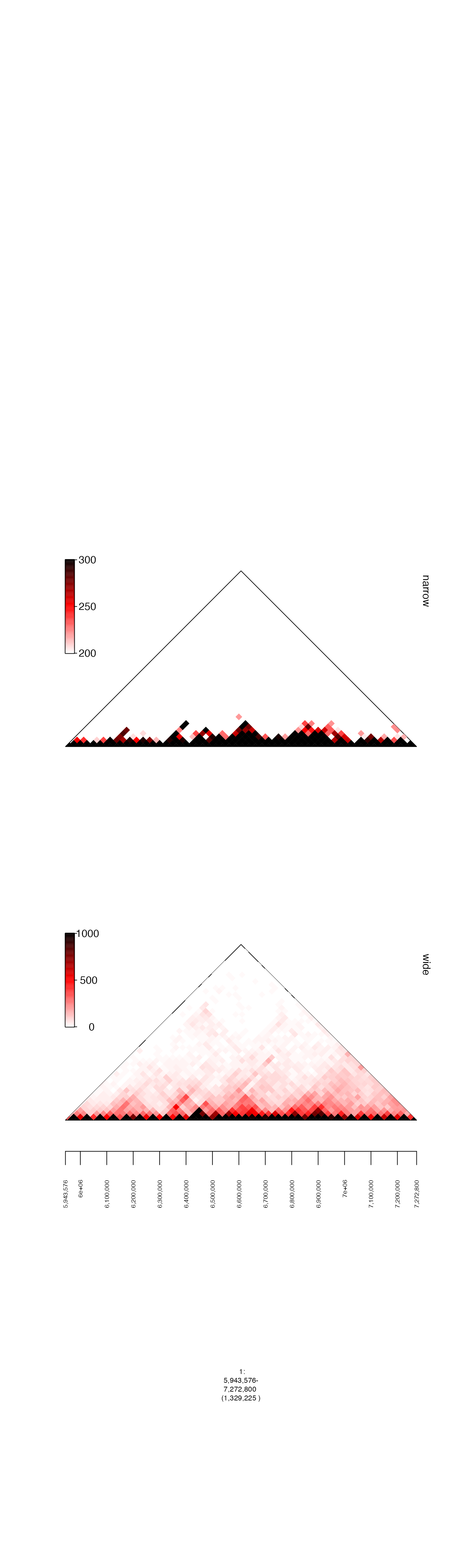
Legends
In some of the examples above, you can see that when we use
gr.colorfield or grl.colorfield a legend is
created to show the mapping of labels to colors. Sometimes, we don’t
want to include a legend in our gTrack. Omitting the legend
is accomplished by setting the parameter legend to
FALSE.
coverage.gr = readRDS(system.file("extdata", "ovcar.subgraph.coverage.rds", package = "gTrack"))
gg = readRDS(system.file("extdata", "ovcar.subgraph.rds", package = "gTrack"))

values(coverage.gr)[, "near_breakend"] = ifelse(coverage.gr %^% (stack(gg$junctions[type == "ALT"]$grl) + 1e4), "yes", "no")

coverage.col.gt = gTrack(coverage.gr, y.field = "cn", circles = TRUE, lwd.border = 0.2, y0 = 0, y1 = 12, gr.colorfield = "near_breakend")
coverage.col.gt$legend = FALSE

fp = parse.gr("1:6043576-7172800")
plot(c(coverage.col.gt, gg$gt), fp + 1e5)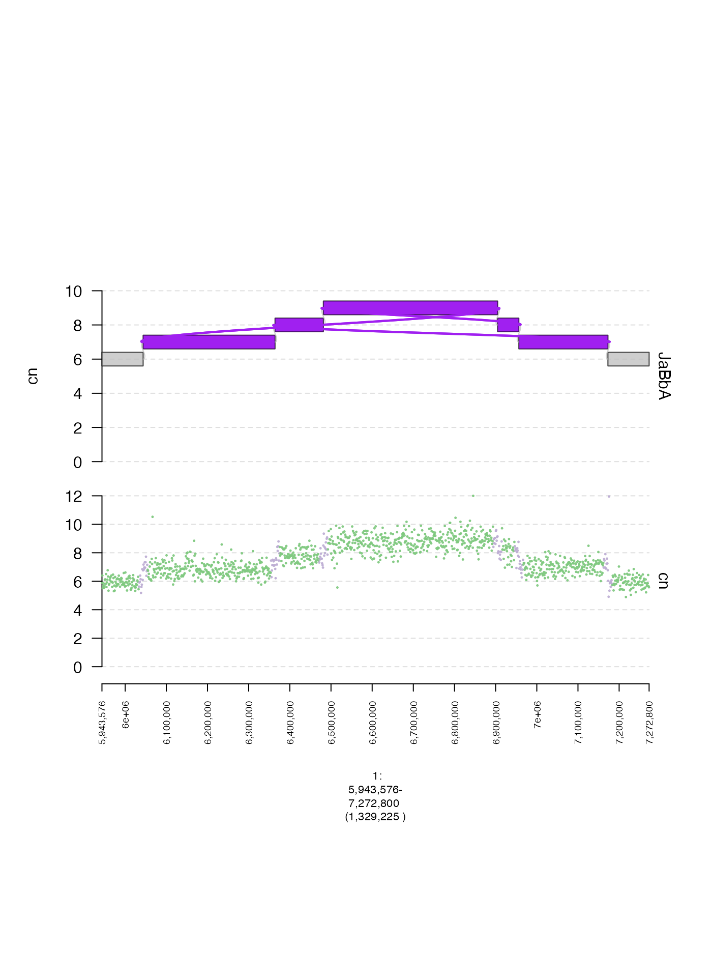
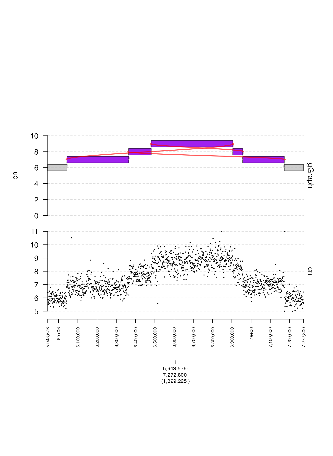
Links
It is possible to plot aberrant adjacencies as a separate track.
These must be supplied to the as a GRangesList to the
links parameter of plot. The length of each
constituent GRanges in this GRangesList should
be 2.
gg = readRDS(system.file("extdata", "ovcar.subgraph.rds", package = "gTrack"))
## create GRangesList corresponding with ALT edges
grl = gg$junctions[type == "ALT"]$grl
plot(c(coverage.gt, gg$gt), fp + 1e5, links = grl)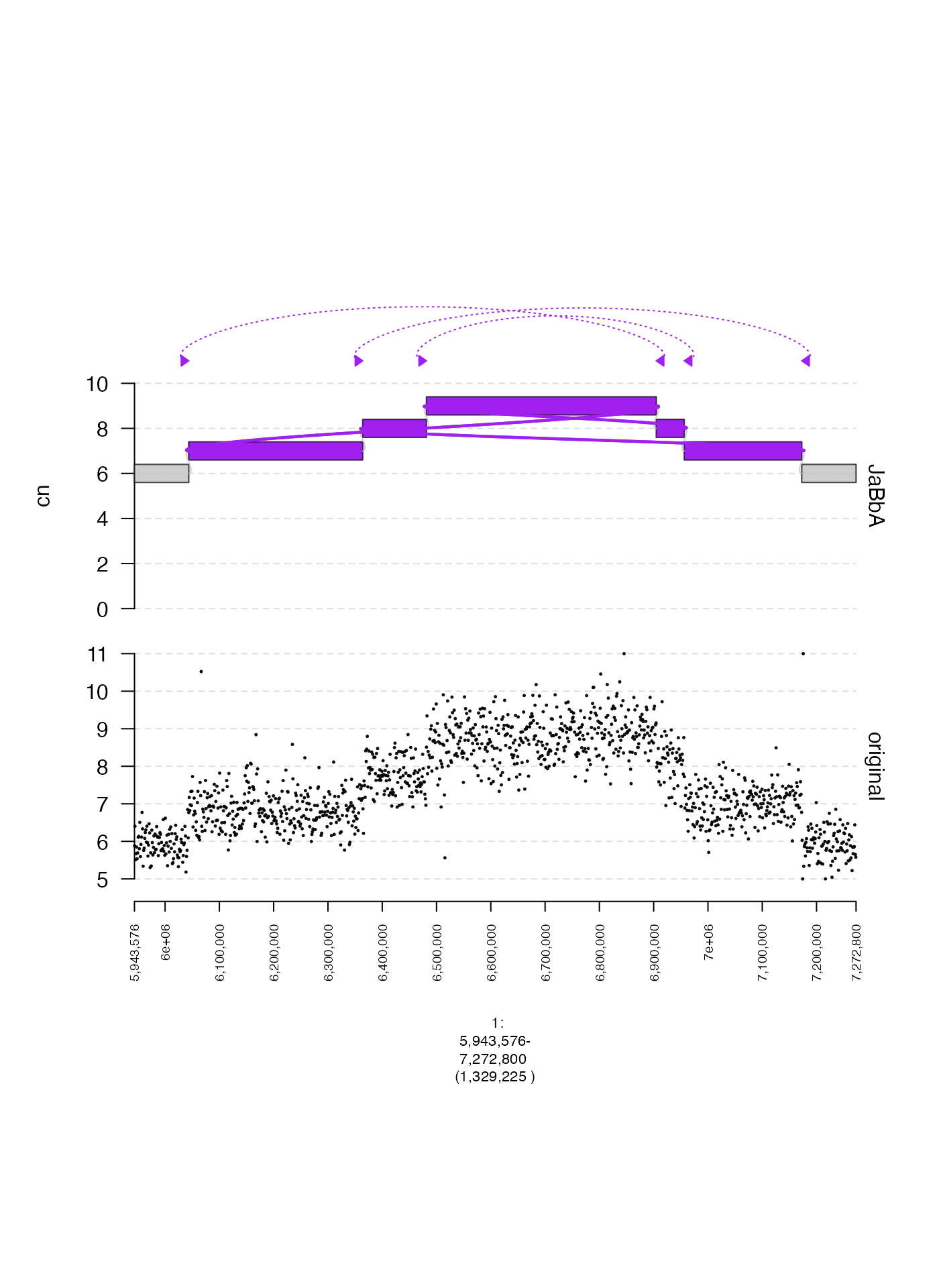
Sequence names with chr prefixes
Some genome assemblies (e.g. GrCh38) have sequence names with a
chr prefix. By default, gTrack strips these
prefixes, but sometimes it is preferable to keep them. This can be done
by setting chr.sub to FALSE in both
plot and gTrack instantiation. An example is
below.
coverage.new = readRDS(system.file("extdata", "ovcar.subgraph.coverage.chr.rds", package = "gTrack"))
gg.new = readRDS(system.file("extdata", "ovcar.subgraph.chr.rds", package = "gTrack"))

chr.fp = gUtils::parse.gr("chr1:6043576-7172800")

gg.gt = gg.new$gtrack(chr.sub = FALSE, y.field = "cn")
gg.gt$y.field = "cn"

chr.coverage.gt = gTrack(coverage.new, y.field = "cn", circles = TRUE, lwd.border = 0.2, chr.sub = FALSE)
grl = gg.new$junctions[type == "ALT"]$grl
plot(c(chr.coverage.gt, gg.gt), chr.fp + 1e5, links = grl, chr.sub = FALSE)